Gradient Descent Strategies | TWO2TWO2TWO2TWO2

Defect of Traditional Gradient Descent

Everyone might know something about the Gradient Descent (GD), which is one of the basic techniques of machine learning. GD is an iteration-based parameter optimizing method. At each iteration, it first calculates the partial derivative of the loss function $J$ with respect to each parameter $c$, and then updates $c$ by:

$c\leftarrow c-\eta \nabla_c$

where the $\eta$ is the learning rate, or the step size. Though simple, GD has some disadvantages to be improved:

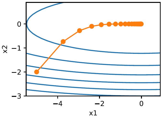
If the parameters are not normalized before training, it is likely to slow down the speed of convergence. The reason is that the learning rates for each parameter are the same. If a parameter is much greater than another parameter, it might get a larger gradient and overshoot. As well, the path to the minimum would oscillate:

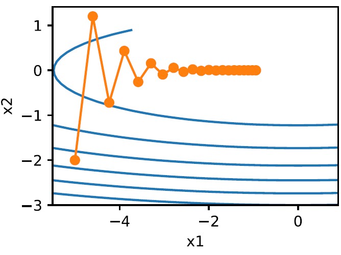
All these will increase the difficulty of training. A simple solution is to set a relatively small learning rate for the model, but it would slow down the training process, which is also not what we expect.
Since the learning rate is invariable, after some iterations, the parameters would reach their minimum. However, if the learning rate is too large, the parameters might “skip” the minimum and fail to converge.

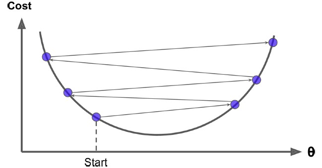
Some parameter optimization algorithms have been proposed to improve these problems. In this article, five ideas to improve GD would be introduced. They are Momentum, Adagrad, RMSProp, Adadelta, and Adam. They are all based on GD, and are still iteration-based, but with some modifications on hyperparameters.

Gradient Descent:

$\begin{aligned} c\leftarrow c-\eta \nabla_c \end{aligned}$

Momentum

The process of GD, especially stochastic gradient descent (SGD) and mini-batch stochastic gradient descent, usually oscillates, resulting in a “winding” path to the minimum.

We denote the updating values for a parameter (omitting the learning rate and the negative sign) at the $n^th$ iteration as $v_n$:

$c\leftarrow c-\eta v_n$

and the gradient as $\nabla_n$. In the traditional gradient descent, the $v_n$ is equal to $\nabla_n$. If we mix into the concept of Momentum, the $v_n$ would be:

$v_n=\beta v_{n-1}+(1-\beta)\nabla_n$

Where $\beta$ is a constant value between 0 and 1. It means that, the updating value of a parameter is changing during the iteration. By unfolding each $v$, we can find that:

$\begin{aligned}v_1&=(1-\beta)\nabla_1\\v_2&=\beta(1-\beta)\nabla_1+(1-\beta)\nabla_2\\v_3&=\beta^2(1-\beta)\nabla_1+\beta(1-\beta)\nabla_2+(1-\beta)\nabla_3\\\cdots\\v_n&=(1-\beta)(\beta^{n-1}\nabla_1+\beta^{n-2}\nabla_2+\cdots+\nabla_n)\end{aligned}$

According to the last equation, $v_n$ is the weighted average of $\nabla_1,\nabla_2,\cdots,\nabla_n$. With Momentum, the direction of the gradient at the current iteration is more similar to the direction of that at the previous iteration. The gradient path seems to be “smoothed”, and oscillates less.

momentum

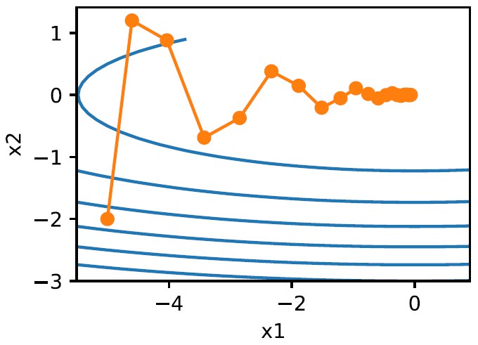
On the other hand, we can imagine the $v$ as the “velocity” of the descendent path. It seems that the $\nabla_n$ for the $v_n$ at the $n^th$ iteration is its “acceleration”, and $v_{n-1}$ is its current velocity. This simulation to physical motion gives gradient descent the “inertia”, and therefore the direction of the gradient varies less. This can help to avoid problems like oscillation and overshooting.

By the way, note that $\frac{1}{1-\beta}\sum_{i=1}^n\beta^{n-i}=1-\beta^n$. Therefore, the sum of weights is approximately equal to 1 when $n$ is big enough. Some versions of Momentum implementation do not have the normalized item $\frac{1}{1-\beta}$, because, after some iterations, its effect of magnifying gradients would be smaller and smaller, so it can be omitted reasonably.

Momentum:

$\begin{aligned} v_n\leftarrow &\beta v_{n-1}+(1-\beta)\nabla_n\\ &c\leftarrow c-\eta v_n \end{aligned}$

Adagrad

To solve the problem caused by the fixed learning rate, one very intuitive solution might be altering the learning rate during the process of gradient descent. Also, intuitively, the learning rate is expected to decrease during the process. If the gradient is too large, the learning rate has to be dropped significantly to ensure the updating value is under control. So, one way to gradually reduce the learning rate is by dividing a variable:

$\begin{aligned}s_n&\leftarrow s_{n-1}+\nabla_n^2\\c\leftarrow &c-\frac{\eta}{\sqrt{s_n+\epsilon}}\nabla_n\end{aligned}$

where the $\epsilon$ is a small constant value for numerical stability. At each iteration, the $s_n$ is added to the square of the gradient, so the denominator of the learning rate increases, keeping reducing the learning rate. If the parameter has a constant and large partial derivative, the learning rate will drop faster for this parameter, while if the gradient of the parameter remains small, its learning rate will decline more slowly. This prevents the model from overshooting while keeping a fast learning speed. The trick is called adaptive learning rate, which is the core idea of Adagrad. However, Adagrad still has some problems. Since the $s_n$ is an accumulation of $\nabla_1$ to $\nabla_n$, at later stages of iteration, the learning rate would become too small for updating, and the descendent path seems like getting “stuck” at the point.

adagrad

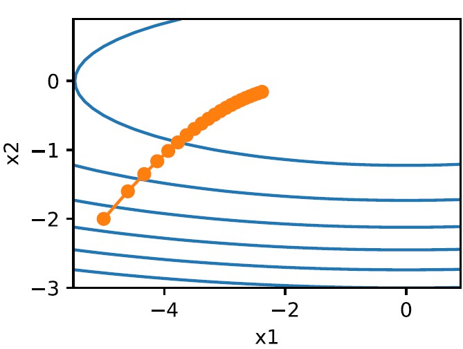
This is due to the unreasonable design of $s$. The next step to perfect the Gradient Descent would be finding a more reliable $s$, which could get rid of the problem of learning rate disappearing.

Adagrad:

$\begin{aligned}s_n&\leftarrow s_{n-1}+\nabla_n^2\\c\leftarrow &c-\frac{\eta}{\sqrt{s_n+\epsilon}}\nabla_n\end{aligned}$

RMSProp

Why not combine the idea of Momentum with the adaptive learning rate together? Because the Momentum is a good method to limit variables from growing infinitely. The $s_n$ is an exponentially weighted average of $\nabla_1^2$ to $\nabla_n^2$, similar to the velocity:

$s_n\leftarrow \gamma s_{n-1}+(1-\gamma)\nabla_n^2$

where $\gamma$ is similar to the $\beta$, a constant value between 0 and 1. As discussed before, the sum of weights is $1-\gamma^n$, so the $s_n$ could not be a too large number to invalidate the learning rate. Even after iterations of gradient descent, the model remains the power to go forward, and finally reaches to the minimum.

rmsprop

RMSProp:

$\begin{aligned} s_n\leftarrow& \gamma s_{n-1}+(1-\gamma)\nabla_n^2\\ c\leftarrow& c-\frac{\eta}{\sqrt{s_n+\epsilon}}\nabla_n \end{aligned}$

Adadelta

RMSProp depends on the learning rate constant $\eta$. The Adadelta method replaces it with a variable which changes during the updating process. Concretely, the learning rate $\eta$ is replaced by:

$\eta\leftarrow \sqrt{\Delta_{n-1}+\epsilon}$

where the $\Delta$ is an exponentially weighted accumulation of the square of the updating value $\nabla’$:

$\begin{aligned} \nabla_n'\leftarrow &\sqrt{\frac{\Delta_{n-1}+\epsilon}{s_n+\epsilon}}\nabla_n\\ \Delta_n\leftarrow& \beta\Delta_{n-1}+(1-\rho)\nabla_n'^2 \end{aligned}$

And finally, update the parameter:

$c\leftarrow c-\nabla_n'$

One of the advantages of the Adadelta is that users do not need to tune the learning rate hyperparameter any more. At the early stages of gradient descent, the gradient is relatively large, and taking larger updating steps by using a greater learning rate is preferred. On contrast, at later stages, the model is close to the minimum, the gradient is not as large as before, and it is better to take smaller steps to approach the minimum. The Adadelta algorithm performs well and is robust during the training process.

Adadelta:

$\begin{aligned} &s_n\leftarrow \gamma s_{n-1}+(1-\gamma)\nabla_n^2\\ &\nabla_n'\leftarrow \sqrt{\frac{\Delta_{n-1}+\epsilon}{s_n+\epsilon}}\nabla_n\\ &\Delta_n\leftarrow \rho\Delta_{n-1}+(1-\rho)\nabla_n'^2\\ &c\leftarrow c-\nabla_n' \end{aligned}$

Adam

As discussed before, $\frac{1}{1-\beta}\sum_{i=1}^n\beta^{n-i}=1-\beta^n$. When $n$ is small, the gradient accumulation from previous steps is small. For example, take $n=1$ and $\beta=0.9$, then the velocity at the first iteration would be $v_1=0.1\nabla_1$, which is much smaller than expected. To avoid slowing training speed at early stages, the $v_n$ is divided by $1-\beta^n$ to rescale:

$\hat{v}_n\leftarrow \frac{v_n}{1-\beta^n}$

After rescaling, the sum of weights becomes 1, which would ensure the model to be trained at a fast speed during the early stages. This trick is called bias correction, which is the main idea of the Adam. Adam combines the momentum, adaptive learning rate, and bias correction. It also corrects the bias of the item $s$:

$\hat{s}_n\leftarrow \frac{s_n}{1-\gamma^n}$

Adam could train models both fast and stable. It performs well and is chosen by many users to optimize parameters.

Adam:

$\begin{aligned} &v_n\leftarrow \beta v_{n-1}+(1-\beta)\nabla_n\\ &\hat{v}_n\leftarrow \frac{v_n}{1-\beta^n}\\ &s_n\leftarrow \gamma s_{n-1}+(1-\gamma)\nabla_n^2\\ &\hat{s}_n\leftarrow \frac{s_n}{1-\gamma^n}\\ &c\leftarrow c-\frac{\eta}{\sqrt{\hat{s}_n+\epsilon}}\hat{v}_n \end{aligned}$

Reference

Dive into Deep Learning
Hands-On Machine Learning with Scikit-Learn and TensorFlow. Aurélien Géron.
Adadelta: an adaptive learning rate method. Matthew D. Zeiler.
Adam: a method for stochastic optimization. Diederik P. Kingma, Jimmy Lei Ba.
CS224n